MNIST with Tensorflow / Keras
MNIST with Tensorflow
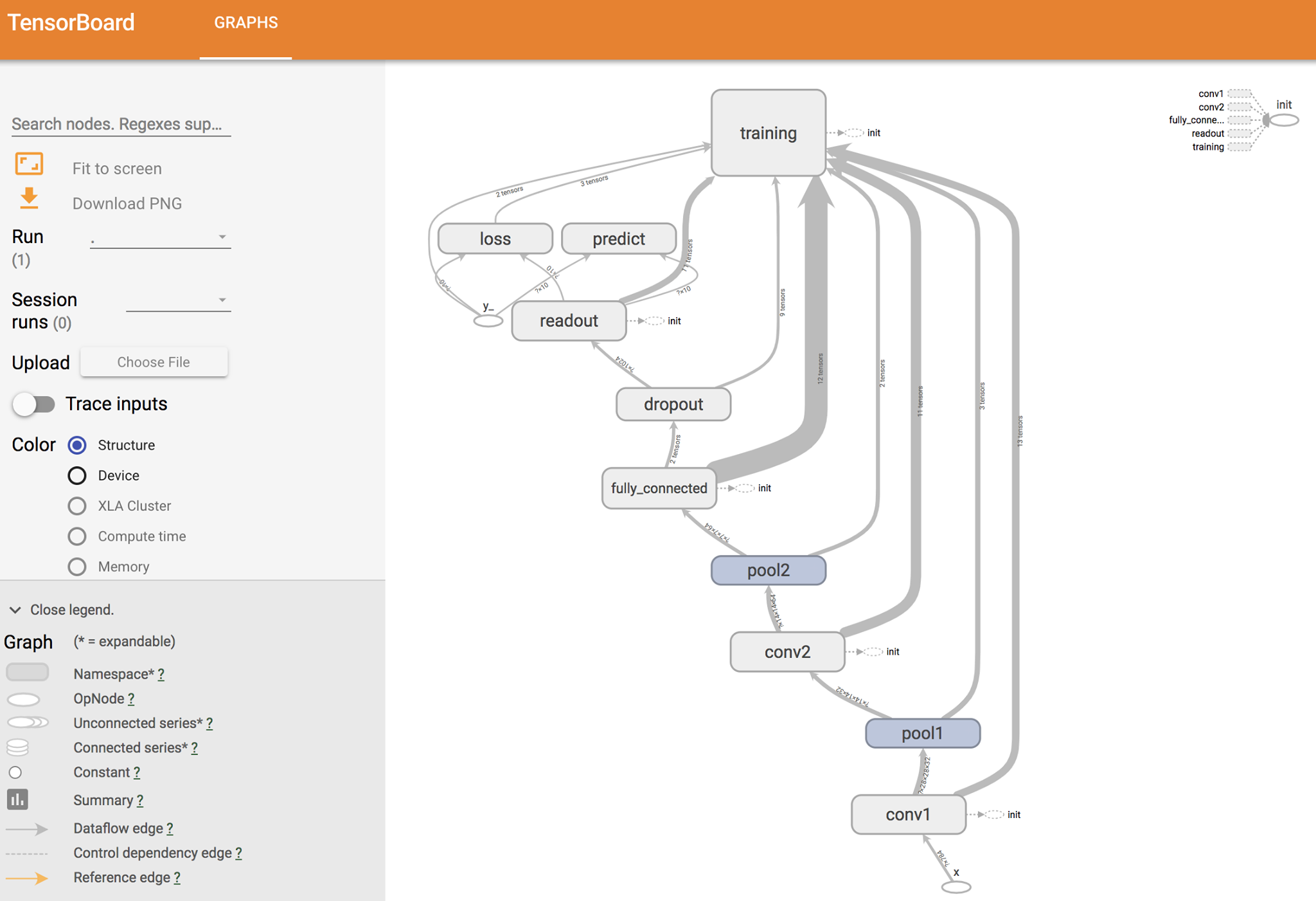
- Tensorflow를 통해 CNN을 활용한 MNIST 학습.
- Tensorboard로 보기 편하게 하기 위해 다음과 같이 진행했습니다.
mport tensorflow as tf
from tensorflow.examples.tutorials.mnist import input_data

#MNIST 데이터 읽어들이기
mnist=input_data.read_data_sets("mnist/", one_hot=True)

pixels=28*28
nums=10 # 0-9사이의 카테고리

#placeholder 정의하기
x=tf.placeholder(tf.float32,shape=(None, pixels), name="x") #image data
y_=tf.placeholder(tf.float32,shape=(None, nums), name="y_") #result label

#가중치와 바이어스를 초기화하는 함수
def weight_variable(name, shape):
    W_init=tf.truncated_normal(shape,stddev=0.1)
    W=tf.Variable(W_init, name="W_"+name)
    return W

def bias_variable(name, size):
    b_init=tf.constant(0,1,shape=[size])
    b=tf.Variable(b_init, name="b_"+name)
    return b

#합성곱 계층을 만드는 함수
def conv2d(x,W):
    return tf.nn.conv2d(x,W,strides=[1,1,1,1], padding='SAME')

#최대 풀링층
def max_pool(x):
    return tf.nn.max_pool(x,ksize=[1,2,2,1], strides=[1,2,2,1],padding='SAME')

#합성곱층1
with tf.name_scope('conv1') as scope:
    W_conv1=weight_variable('conv1',[5,5,1,32]) # 5*5 filter, 입력 채녈 1 (흑백), 출력 채녈 32
    b_conv1=bias_variable('conv1',32)
    x_image=tf.reshape(x,[-1,28,28,1])
    h_conv1=tf.nn.relu(conv2d(x_image, W_conv1)+b_conv1)

#풀링층1
with tf.name_scope('pool1') as scope:
    h_pool1=max_pool(h_conv1)

#합성곱층2
with tf.name_scope('conv2') as scope:
    W_conv2=weight_variable('conv2', [5,5,32,64])
    b_conv2=bias_variable('conv2', 64)
    h_conv2=tf.nn.relu(conv2d(h_pool1, W_conv2) + b_conv2)

#풀링층2
with tf.name_scope('pool2') as scope:
    h_pool2=max_pool(h_conv2)

#fully connected
with tf.name_scope('fully_connected') as scope:
    n=7*7*64 #2*2 pooling 2번 = 28/2/2 -> 7*7
    W_fc=weight_variable('fc', [n,1024])
    b_fc=bias_variable('fc', 1024)
    h_pool2_flat=tf.reshape(h_pool2, [-1,n])
    h_fc=tf.nn.relu(tf.matmul(h_pool2_flat, W_fc)+b_fc)

#dropout
with tf.name_scope('dropout') as scope:
    keep_prob=tf.placeholder(tf.float32)
    h_fc_drop=tf.nn.dropout(h_fc, keep_prob)

#출력층
with tf.name_scope('readout') as scope:
    W_fc2=weight_variable('fc2', [1024,10])
    b_fc2=bias_variable('fc2',10)
    y_conv=tf.nn.softmax(tf.matmul(h_fc_drop, W_fc2)+b_fc2)

#모델 학습시키기
with tf.name_scope('loss') as scope:
    cross_entoropy=-tf.reduce_sum(y_*tf.log(y_conv))
with tf.name_scope('training') as scope:
    optimizer=tf.train.AdamOptimizer(1e-4) # 확률적 SGD
    train_step=optimizer.minimize(cross_entoropy)

#모델 평가하기
with tf.name_scope('predict') as scope:
    predict_step=tf.equal(tf.argmax(y_conv,1), tf.argmax(y_,1))
    accuracy_step=tf.reduce_mean(tf.cast(predict_step, tf.float32))

#feed_dict 설정하기
def set_feed(images,labels, prob):
    return {x:images, y_:labels, keep_prob: prob}

#세션 시작하기
with tf.Session() as sess:
    sess.run(tf.global_variables_initializer())
    #Tensorboard
    tw=tf.summary.FileWriter("log_dir",graph=sess.graph)
    #test 전용 피드
    test_fd=set_feed(mnist.test.images, mnist.test.labels,1)
    #학습시작
    for step in range(10000):
        batch=mnist.train.next_batch(50) #50개 이미지 10000번 학습
        fd=set_feed(batch[0], batch[1], 0.5)
        _, loss=sess.run([train_step, cross_entoropy], feed_dict=fd)
        if step % 100 ==0:
            acc=sess.run(accuracy_step,feed_dict=test_fd)
            print("step=", step, " loss=", loss, " acc=", acc)

    #최종결과출력
    acc=sess.run(accuracy_step, feed_dict=test_fd)
    print("정답률=",acc)
step= 0  loss= 343.45953  acc= 0.1128
step= 100  loss= 45.32565  acc= 0.8844
step= 200  loss= 23.790255  acc= 0.9213
step= 300  loss= 24.37558  acc= 0.9388
step= 400  loss= 8.762227  acc= 0.9466
step= 500  loss= 5.5240602  acc= 0.9522
...
step= 9500  loss= 0.036732152  acc= 0.9911
step= 9600  loss= 0.93421096  acc= 0.9904
step= 9700  loss= 1.8589059  acc= 0.9912
step= 9800  loss= 0.20325959  acc= 0.9916
step= 9900  loss= 1.7240194  acc= 0.9908
정답률= 0.9913
MNIST with Keras
- Keras를 사용해 MNIST 분류
from keras.datasets import mnist
from keras.models import Sequential
from keras.layers.core import Dense, Dropout, Activation
from keras.callbacks import EarlyStopping
from keras.optimizers import Adam
from keras.utils import np_utils

#Mnist data 불러오기
(X_train, y_train),(X_test,y_test)=mnist.load_data()

#데이터를 float32 자료형 변환, 정규화
X_train = X_train.reshape(60000,784).astype('float32')
X_test=X_test.reshape(10000,784).astype('float32')
X_train/=255 #pixel 데이터 정규화 (각 색 농도가 0~255까지 있다)
X_test/=255

#레이블 데이터를 0-9까지 카테고리 배열로 변환
y_train=np_utils.to_categorical(y_train, 10) #10차원 배열 데이터로 변환
y_test=np_utils.to_categorical(y_test, 10)

#모델 구조 정의하기
model=Sequential()
model.add(Dense(512,input_shape=(784,)))
model.add(Activation('relu'))
model.add(Dropout(0.2))
model.add(Dense(512))
model.add(Activation('relu'))
model.add(Dropout(0.2))
model.add(Dense(10))
model.add(Activation('softmax'))

#모델 구축하기
model.compile(
    loss='categorical_crossentropy',
    optimizer=Adam(),
    metrics=['accuracy'])

#데이터 훈련하기
hist=model.fit(
    X_train, y_train,
    batch_size=100, #한번에 처리하는 사진 장 수
    nb_epoch=20, #전체 데이터셋 반복횟수
    validation_split=0.1,
    callbacks=[EarlyStopping(monitor='val_loss',patience=2)],
    verbose=1)

#테스트 데이터로 평가하기
score=model.evaluate(X_test, y_test, verbose=1)
print("loss=",score[0])
print("accuracy=",score[1])
Train on 54000 samples, validate on 6000 samples
Epoch 1/20
54000/54000 [==============================] - 10s 177us/step - loss: 0.2530 - acc: 0.9232 - val_loss: 0.0956 - val_acc: 0.9715
Epoch 2/20
54000/54000 [==============================] - 8s 152us/step - loss: 0.1058 - acc: 0.9674 - val_loss: 0.0856 - val_acc: 0.9740
Epoch 3/20
54000/54000 [==============================] - 10s 178us/step - loss: 0.0751 - acc: 0.9764 - val_loss: 0.0831 - val_acc: 0.9757
Epoch 4/20
54000/54000 [==============================] - 10s 178us/step - loss: 0.0605 - acc: 0.9808 - val_loss: 0.0835 - val_acc: 0.9775
Epoch 5/20
54000/54000 [==============================] - 9s 162us/step - loss: 0.0480 - acc: 0.9846 - val_loss: 0.0741 - val_acc: 0.9793
Epoch 6/20
54000/54000 [==============================] - 11s 204us/step - loss: 0.0425 - acc: 0.9866 - val_loss: 0.0699 - val_acc: 0.9803
Epoch 7/20
54000/54000 [==============================] - 11s 199us/step - loss: 0.0364 - acc: 0.9878 - val_loss: 0.0716 - val_acc: 0.9808
Epoch 8/20
54000/54000 [==============================] - 10s 185us/step - loss: 0.0326 - acc: 0.9892 - val_loss: 0.0772 - val_acc: 0.9820
10000/10000 [==============================] - 1s 79us/step
loss= 0.08363286133202345
accuracy= 0.9791